Linear Regression from Text
data preprocessing
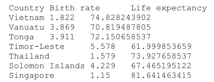
def read_birth_life_data(filename):
    """
    Read in birth_life_2010.txt and return:
    data in the form of NumPy array
    n_samples: number of samples
    """
    text = open(filename, 'r').readlines()[1:]
    data = [line[:-1].split('\t') for line in text]
    births = [float(line[1]) for line in data]
    lifes = [float(line[2]) for line in data]
    data = list(zip(births, lifes))
    n_samples = len(data)
    data = np.asarray(data, dtype=np.float32)
    return data, n_samples

data, n_samples = read_birth_life_data(DATA_FILE)
Dataset 만들기 - batch size : 1
dataset = tf.data.Dataset.from_tensor_slices((data[:,:1], data[:,1:]))
dataset = dataset.shuffle(n_samples).batch(1)
Keras Sequential API 사용하여 model 만들기
keras.laysers.Dense API는 1개의 linear layer를 만들어주고 내부에서 weight와 bias를 자동으로 생성
## linear regression model function
def create_model():
    ## Sequential API 사용
    model = keras.Sequential()
    ## keras.layers.Dense layer - units는 output의 수를 의미함
    ## sequential model의 첫번째 layer에는 input_shape을 써줌
    model.add(keras.layers.Dense(units=1, input_shape=(1,)))
    return model

## model 생성
model = create_model()
model.summary()
Model: "sequential"
_________________________________________________________________
Layer (type) Output Shape Param #
=================================================================
dense (Dense) (None, 1) 2
=================================================================
Total params: 2
Trainable params: 2
Non-trainable params: 0## loss function - Mean Squared Error
def compute_loss(labels, predictions):
return tf.reduce_mean(tf.square(labels - predictions))
## learning rate & optimizer
learning_rate = 0.001
optimizer = tf.keras.optimizers.SGD(learning_rate=learning_rate)
## gradient 계산하여 gradient descent 학습법으로 weight와 bias update
def train_on_batch(model, x, y):
with tf.GradientTape() as tape:
predictions = model(x)
loss = compute_loss(y, predictions)
grads = tape.gradient(loss, model.trainable_variables)
optimizer.apply_gradients(grads_and_vars=zip(grads, model.trainable_variables))
return lossTraining with stochastic gradient descent
import time
t0 = time.time()

n_epoch = 100
for epoch in range(n_epoch):
    total_loss = 0.
    for x, y in dataset:
        loss = train_on_batch(model, x, y)
        total_loss += loss
    print('Epoch {0}: {1}'.format(epoch+1, total_loss/n_samples))

t_end = time.time() - t0
print('epoch당 걸린 시간: %.3f 초' % (t_end / n_epoch))
#### 결과 확인
w = model.trainable_variables[0]
b = model.trainable_variables[1]
plt.plot(data[:,0], data[:,1], 'bx', label='Real data')
plt.plot(data[:,0], data[:,[0]] * w.numpy() + b.numpy(), 'y', label='Predicted data')
plt.legend()
plt.show()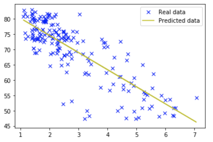
Autograph를 이용한 속도 향상
학습 함수를 정적 그래프로 컴파일 해 봅시다. 이를 위해서 해야할 것은 문자 그대로, tf.function이라는 데코레이터를 위에 넣어주는것 뿐입니다
autograph를 이용하여 static graph로 compile
@tf.function
def train_on_batch(model, x, y):
    with tf.GradientTape() as tape:
        predictions = model(x)
        loss = compute_loss(y, predictions)
    grads = tape.gradient(loss, model.trainable_variables)
    optimizer.apply_gradients(grads_and_vars=zip(grads, model.trainable_variables))
    return loss
Training with stochastic gradient descent
t0 = time.time()

n_epoch = 100
for epoch in range(n_epoch):
    total_loss = 0.
    for x, y in dataset:
        loss = train_on_batch(model, x, y)
        total_loss += loss
    print('Epoch {0}: {1}'.format(epoch+1, total_loss/n_samples))

t_end = time.time() - t0
print('epoch당 걸린 시간: %.3f 초' % (t_end / n_epoch))
Linear Regression using Keras Training API
## Dataset 만들기 - batch size : 10
batch_size = 10
dataset = tf.data.Dataset.from_tensor_slices((data[:,:1], data[:,1:]))
dataset = dataset.shuffle(n_samples).batch(batch_size).repeat()
## linear regression model function
def create_model():
## Sequential API 사용
model = keras.Sequential()
## keras.layers.Dense layer - units는 output의 수를 의미함
## sequential model의 첫번째 layer에는 input_shape을 써줌
model.add(keras.layers.Dense(units=1, input_shape=(1,)))
return model## model 생성
model = create_model()
## summary 확인
model.summary()model.compile()을 이용하여, loss funtion과 optimizer, 평가 metric을 정의할 수 있음
## model compile
learning_rate = 0.01
model.compile(optimizer=keras.optimizers.SGD(learning_rate),
loss='MSE',
metrics=['MSE'])## 한 epoch이 몇 개의 batch(step)로 구성되는지 계산
steps_per_epoch = n_samples // batch_size
n_epoch = 100
t0 = time.time()
history = model.fit(dataset, epochs=n_epoch, steps_per_epoch=steps_per_epoch)
t_end = time.time() - t0
print('epoch당 걸린 시간: %.3f 초' % (t_end / n_epoch))## 결과 확인
w = model.trainable_variables[0]
b = model.trainable_variables[1]
plt.plot(data[:,0], data[:,1], 'bx', label='Real data')
plt.plot(data[:,0], data[:,[0]] * w.numpy() + b.numpy(), 'r', label='Predicted data')
plt.legend()
plt.show()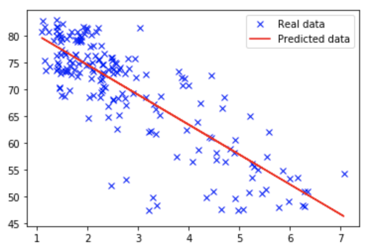
Logistic Regression
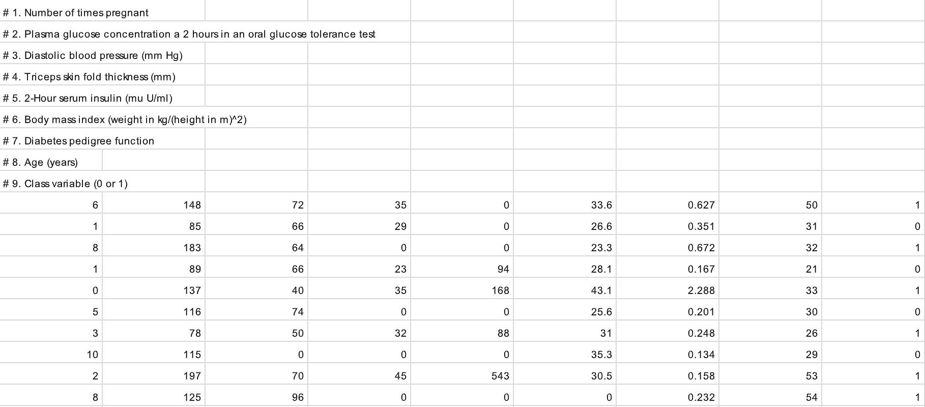
Pima Indians Diabetes Dataset for Binary Classification
This dataset describes the medical records for Pima Indians and whether or not each patient will have an onset of diabetes within five years.
- 인스턴스 수 : 768개
- 속성 수 : 8가지
- 클래스 수 : 2가지
8가지 속성(1번~8번)과 결과(9번)의 상세 내용
- 임신 횟수
- 경구 포도당 내성 검사에서 2시간 동안의 혈장 포도당 농도
- 이완기 혈압 (mm Hg)
- 삼두근 피부 두겹 두께 (mm)
- 2 시간 혈청 인슐린 (mu U/ml)
- 체질량 지수
- 당뇨 직계 가족력
- 나이 (세)
- 5년 이내 당뇨병이 발병 여부
## input file 읽기
xy = np.loadtxt(DATA_FILE, delimiter=',', dtype=np.float32)
x_train = xy[:, 0:-1]
y_train = xy[:, [-1]]
## data preprocessing을 위한 minmax scaler
def MinMaxScaler(data):
''' Min Max Normalization
Parameters
----------
data : numpy.ndarray
input data to be normalized
shape: [Batch size, dimension]
Returns
----------
data : numpy.ndarry
normalized data
shape: [Batch size, dimension]
References
----------
.. [1] http://sebastianraschka.com/Articles/2014_about_feature_scaling.html
'''
numerator = data - np.min(data, 0)
denominator = np.max(data, 0) - np.min(data, 0)
# noise term prevents the zero division
return numerator / (denominator + 1e-7)
## data preprocessing
x_train = MinMaxScaler(x_train)Hyper parameter 설정
## batch size, epoch, learning rate
n_data = x_train.shape[0]
batch_size = x_train.shape[0]
n_epoch = 1000
learning_rate = 0.4
## dataset 만들기
dataset = tf.data.Dataset.from_tensor_slices((x_train, y_train)).shuffle(1000).batch(batch_size).repeat()
## model 만들기
def create_model():
model = keras.Sequential()
model.add(keras.layers.Dense(units=1, activation='sigmoid', input_shape=(8,)))
return model
## model 생성
model = create_model()
## summary 확인
model.summary()model compile
1-class logistic regression이므로 loss는 binary cross-entropy 사용, metric은 accuracy
model.compile(optimizer=keras.optimizers.SGD(learning_rate),
             loss='binary_crossentropy',
             metrics=['accuracy'])

## 한 epoch이 몇 개의 batch(step)로 구성되는 지 계산
steps_per_epoch = n_data // batch_size

## Training
history = model.fit(dataset, epochs=n_epoch, steps_per_epoch=steps_per_epoch)
accuracy 확인
model.evaluate은 정답이 있는 data의 경우(validation set) 결과를 확인할 때 사용함
model.evaluate(dataset, steps=steps_per_epoch)## 정답이 없는 data(test set)의 경우에는 model.predict 사용
model.predict(dataset, steps=steps_per_epoch)## model.fit, evaluate, predict는 dataset이 아닌 data도 직접 입력으로 받을 수 있음
model = create_model()
model.compile(optimizer=keras.optimizers.SGD(learning_rate),
loss='binary_crossentropy',
metrics=['accuracy'])
model.evaluate(x_train, y_train)
model.fit(x_train, y_train, batch_size=batch_size, epochs=n_epoch)
model.evaluate(x_train, y_train)n번째 data에 대한 예측값
import random
n = random.randrange(n_data)
prediction = model.predict(x_train[[n]])
print(prediction)

## n번째 data에 대한 정답
label = y_train[n]
print(label)

if (prediction>=0.5) == label:
    print("correct prediction")
else:
    print("wrong prediction")
[[0.567724]]
[1.]
correct prediction'DEEP LEARNING > Tensorflow Training' 카테고리의 다른 글
| cnn 실습_나만의 이미지 데이터를 만들고 학습하기(3) - functional API & save_model (0) | 2020.03.26 |
|---|---|
| cnn 실습_나만의 이미지 데이터를 만들고 학습하기(2) - sequential API (0) | 2020.03.21 |
| cnn 실습_나만의 이미지 데이터를 만들고 학습하기(1) - image crawling (0) | 2020.03.20 |
| Make A Dataset (0) | 2020.02.26 |
| Basic (0) | 2020.02.24 |

